panGenomeBreedr_Workflows

Table of contents

• Variant Discovery
  • Pangenome Data and Database Rationale
  • Recommended Schema for the SQLite Database
  • Database Creation
  • Query Variant Tables
  • Filter Variants by Allele Frequency
  • Summarize SnpEff Annotation and Impact
• KASP Marker Design
• KASP Marker Validation
• Decision Support for Trait Introgression and MABC
  • Creating Heatmaps with panGB
  • Trait Introgression Hypothesis Testing
  • Decision Support for MABC
  • Weighted RPP computation in panGB
  • Decision Support for Foreground Selection

Variant Discovery

Pangenome Data and Database Rationale

The examples used in this documentation are based on sorghum pangenome resources derived from whole-genome resequencing data of 1,676 sorghum lines. Variant calling was performed using version v5.1 of the BTx623 reference genome. The resulting SNP and INDEL variants were functionally annotated using snpEff.

Direct querying of snpEff-annotated VCF files from R is often computationally slow and inefficient, especially with large datasets. To overcome this limitation, we built a SQLite database that stores the variants, annotations, and genotypes in normalized tables. This structure allows for fast and flexible access to relevant data, supporting workflows for trait-predictive marker discovery.

We strongly recommend the creation of similar databases for other crops. The SQLite format offers a compact, portable, and queryable representation of pangenome-derived variant data, significantly improving performance and reproducibility in variant discovery pipelines.

A compressed format of the SQLite database for sorghum can be downloaded here.

Recommended Schema for the SQLite Database

The SQLite database contains the following three key tables:

variants

This table stores core metadata variant information extracted from the VCF.

Column	Description
variant_id	Unique variant identifier
chrom	Chromosome name
pos	Genomic position (1-based)
ref	Reference allele
alt	Alternate allele
variant_type	Type of variant (e.g., SNP, indel)

annotations

This table contains functional annotations from snpEff, typically including predicted effects, gene names, and functional categories.

Column	Description
variant_id	Foreign key linking to variants
gene_name	Sorghum gene ID (e.g., “Sobic.005G213600”)
effect	Type of effect (e.g., missense_variant)
impact	snpEff predicted impact (e.g., HIGH)
feature_type	Type of annotated feature (e.g., exon)
…	Additional snpEff annotation fields

genotypes

This table stores genotype calls per sample for each variant in a wide format.

Column	Description
variant_id	Foreign key linking to variants
chrom	Chromosome name
pos	Genomic position
sample1	Genotype for Sample 1 (e.g., 1|1)
sample2	Genotype for Sample 2 (e.g., 0|0)
…	Genotypes for other samples

Database Creation

We generated the SQLite database using a custom workflow that

1. Parses a multi-sample VCF file annotated by snpEff,
2. Extracts variant, annotation, and genotype data,
3. Writes the data into normalized relational tables (variants, annotations, genotypes).

A prebuilt mini example database (mini_sorghum_variant_vcf.db.gz) is included in the extdata/ folder of the package.

Query Variant Tables

The query_db() function allows users to query specific tables within a panGenomeBreedr-formatted SQLite database for variants, annotations, or genotypes based on chromosome coordinates or candidate gene IDs.

This function retrieves records from one of the following tables in the database:

• variants: Basic variant information (chromosome, position, REF/ALT alleles, etc.)
• annotations: Variant effect predictions (e.g., from snpEff)
• genotypes: Genotypic data across lines/samples plus the metadata of the variants.

Users can specify genomic coordinates (chrom, start, end) or a candidate gene name (gene_name) to extract relevant entries.

If used correctly, the query_db() function returns a data frame containing the filtered records from the selected table.

library(panGenomeBreedr)

# This example uses the mini SQLite database included in the package.
# Define a temporary path and decompress the example database
path <- tempdir()
mini_db <- system.file("extdata", "mini_sorghum_variant_vcf.db.gz",
                       package = "panGenomeBreedr", mustWork = TRUE)
mini_db_path <- file.path(path, 'mini_sorghum_variant_vcf.db')
R.utils::gunzip(mini_db, destname = mini_db_path, remove = FALSE)

# Query VCF genotypes within the genomic range: Chr05:75104537-75106403
gt_region <- query_db(db_path = mini_db_path,
                      chrom = "Chr05",
                      start = 75104537,
                      end = 75106403,
                      table_name = "genotypes")

# Query snpEff annotations within a candidate gene
annota_region <- query_db(db_path = mini_db_path,
                          chrom = "Chr05",
                          start = 75104537,
                          end = 75106403,
                          table_name = "annotations",
                          gene_name = "Sobic.005G213600")

# Clean up temporary files
unlink(list.files(tempdir(), full.names = TRUE, recursive = TRUE), 
       recursive = TRUE)

Table 1: Queried genotypes for varaints from the SQLite database.

variant_id	chrom	pos	variant_type	ref	alt	IDMM	ISGC	ISGK	ISHC
INDEL_Chr05_75104541	Chr05	75104541	INDEL	T	TGAC	0|0	0|0	0|0	0|0
SNP_Chr05_75104557	Chr05	75104557	SNP	C	T	0|0	0|0	0|0	0|0
SNP_Chr05_75104560	Chr05	75104560	SNP	C	T	0|0	0|0	0|0	0|0
INDEL_Chr05_75104564	Chr05	75104564	INDEL	C	CA	0|0	0|0	0|0	0|0
SNP_Chr05_75104568	Chr05	75104568	SNP	G	T	0|0	0|0	0|0	0|0

Table 2: Queried annotations for variants from the SQLite database.

	variant_id	allele	annotation	impact	gene_name	gene_id	feature_type	feature_id	transcript_biotype	rank	HGVS_c	HGVS_p	chrom	pos
1	INDEL_Chr05_75104541	TGAC	3_prime_UTR_variant	MODIFIER	Sobic.005G213600	Sobic.005G213600.v5.1	transcript	Sobic.005G213600.1.v5.1	protein_coding	2/2	c.322_324dupGTC		Chr05	75104541
4	SNP_Chr05_75104557	T	3_prime_UTR_variant	MODIFIER	Sobic.005G213600	Sobic.005G213600.v5.1	transcript	Sobic.005G213600.1.v5.1	protein_coding	2/2	c.*309G>A		Chr05	75104557
7	SNP_Chr05_75104560	T	3_prime_UTR_variant	MODIFIER	Sobic.005G213600	Sobic.005G213600.v5.1	transcript	Sobic.005G213600.1.v5.1	protein_coding	2/2	c.*306G>A		Chr05	75104560
10	INDEL_Chr05_75104564	CA	3_prime_UTR_variant	MODIFIER	Sobic.005G213600	Sobic.005G213600.v5.1	transcript	Sobic.005G213600.1.v5.1	protein_coding	2/2	c.*301dupT		Chr05	75104564
13	SNP_Chr05_75104568	T	3_prime_UTR_variant	MODIFIER	Sobic.005G213600	Sobic.005G213600.v5.1	transcript	Sobic.005G213600.1.v5.1	protein_coding	2/2	c.*298C>A		Chr05	75104568

Summarize SnpEff Annotation and Impact

The query_ann_summary() function provides a convenient way to summarize the distribution of SnpEff annotations and impact categories across variant types (e.g., SNPs, indels) within a defined genomic region.

This function enables users to quickly assess the types and functional implications of variants located within candidate genes or genomic intervals of interest.

library(panGenomeBreedr)

# Prepare test database
path <- tempdir()
mini_db <- system.file("extdata", "mini_sorghum_variant_vcf.db.gz",
                       package = "panGenomeBreedr", mustWork = TRUE)
mini_db_path <- file.path(path, 'mini_sorghum_variant_vcf.db')
R.utils::gunzip(mini_db, destname = mini_db_path, remove = FALSE)

# Run annotation summary for region Chr05:75104537-75106403
ann_summary <- query_ann_summary(db_path = mini_db_path,
                                 chrom = "Chr05",
                                 start = 75104537,
                                 end = 75106403)
# Clean up
unlink(list.files(tempdir(), full.names = TRUE, recursive = TRUE), 
       recursive = TRUE)

Annotation summary for variants within the genomic range.

	annotation	variant_type	count
24	upstream_gene_variant	SNP	149
12	upstream_gene_variant	INDEL	53
19	downstream_gene_variant	SNP	46
22	missense_variant	SNP	29
23	synonymous_variant	SNP	21
13	3_prime_UTR_variant	SNP	18

Functional impact summary for variants within the genomic range.

	impact	variant_type	count
8	MODIFIER	SNP	220
4	MODIFIER	INDEL	82
7	MODERATE	SNP	29
6	LOW	SNP	21
1	HIGH	INDEL	6
3	MODERATE	INDEL	5

The query_ann_summary() function returns a list with the following elements:

• annotation_summary: Data frame summarizing the count of each SnpEff annotation grouped by variant type.

• impact_summary: Data frame summarizing the count of each SnpEff impact level (e.g., HIGH, MODERATE) grouped by variant type.

• variant_type_totals: Total count of variants in the region grouped by variant type.

The annotation summary shows that there are six (6) INDEL variants with a HIGH impact on protein function. To see these variants, we need to use the query_by_impact() function, as shown below:

# Prepare test database
path <- tempdir()
mini_db <- system.file("extdata", "mini_sorghum_variant_vcf.db.gz",
                       package = "panGenomeBreedr", mustWork = TRUE)
mini_db_path <- file.path(path, 'mini_sorghum_variant_vcf.db')
R.utils::gunzip(mini_db, destname = mini_db_path, remove = FALSE)

# Extract HIGH impact variant for a region or gene
high_variants <- query_by_impact(db_path = mini_db_path,
                                impact_level = 'high',
                                chrom = "Chr05",
                                start = 75104537,
                                end = 75106403)

# Clean up
unlink(list.files(tempdir(), full.names = TRUE, recursive = TRUE), 
       recursive = TRUE)

HIGH impact variants within a defined genomic range.

variant_id	chrom	pos	ref	alt	qual	filter	variant_type	allele	annotation	impact	gene_name	gene_id	feature_type	feature_id	transcript_biotype	rank	HGVS_c	HGVS_p
INDEL_Chr05_75104881	Chr05	75104881	G	GTCGA	.	PASS	INDEL	GTCGA	frameshift_variant	HIGH	Sobic.005G213600	Sobic.005G213600.v5.1	transcript	Sobic.005G213600.1.v5.1	protein_coding	2/2	c.1343_1344insTCGA	p.Ser449fs
INDEL_Chr05_75105587	Chr05	75105587	GC	G	.	PASS	INDEL	G	frameshift_variant	HIGH	Sobic.005G213600	Sobic.005G213600.v5.1	transcript	Sobic.005G213600.1.v5.1	protein_coding	2/2	c.637delG	p.Ala213fs
INDEL_Chr05_75105598	Chr05	75105598	GT	G	.	PASS	INDEL	G	frameshift_variant	HIGH	Sobic.005G213600	Sobic.005G213600.v5.1	transcript	Sobic.005G213600.1.v5.1	protein_coding	2/2	c.626delA	p.Asp209fs
INDEL_Chr05_75106156	Chr05	75106156	CGTAT	C	.	PASS	INDEL	C	frameshift_variant	HIGH	Sobic.005G213600	Sobic.005G213600.v5.1	transcript	Sobic.005G213600.1.v5.1	protein_coding	2/2	c.65_68delATAC	p.His22fs
INDEL_Chr05_75106295	Chr05	75106295	A	ATC	.	PASS	INDEL	ATC	frameshift_variant	HIGH	Sobic.005G213600	Sobic.005G213600.v5.1	transcript	Sobic.005G213600.1.v5.1	protein_coding	1/2	c.38_39dupGA	p.Ser14fs
INDEL_Chr05_75106325	Chr05	75106325	G	GTA	.	PASS	INDEL	GTA	frameshift_variant	HIGH	Sobic.005G213600	Sobic.005G213600.v5.1	transcript	Sobic.005G213600.1.v5.1	protein_coding	1/2	c.8_9dupTA	p.Gln4fs

Filter Variants by Allele Frequency

The query_by_af() and filter_by_af() functions allow users to filter queried variants based on alternate allele frequency thresholds within a specified genomic region.

This is particularly useful for identifying polymorphic sites within candidate gene regions or windows of interest that meet desired minor allele frequency (MAF) thresholds for marker development.

An example usage for the filter_by_af() function is shown in the code snippet below:

library(panGenomeBreedr)

# Define temporary directory and decompress demo database
path <- tempdir()
mini_db <- system.file("extdata", "mini_sorghum_variant_vcf.db.gz",
                       package = "panGenomeBreedr", mustWork = TRUE)
mini_db_path <- file.path(path, 'mini_sorghum_variant_vcf.db')
R.utils::gunzip(mini_db, destname = mini_db_path, remove = FALSE)

# Extract genotype data for all HIGH impact variants and filter by alternate allele frequency
geno_high_filtered <- query_genotypes(db_path = mini_db_path,
                                      variant_ids = high_variants$variant_id,
                                      meta_data = c('chrom', 'pos', 'ref', 'alt', 'variant_type')) |>
  
  filter_by_af(min_af = 0.05)

Table 3: Filtered variants from the SQLite database.

	variant_id	chrom	pos	ref_af	alt_af
1	INDEL_Chr05_75104881	Chr05	75104881	0.9495823	0.0504177
4	INDEL_Chr05_75106156	Chr05	75106156	0.9474940	0.0525060
5	INDEL_Chr05_75106295	Chr05	75106295	0.9439141	0.0560859

# Get genotype data for HIGH impact variants that passed allele filter
geno_high_filtered <- query_genotypes(db_path = mini_db_path,
                                      variant_ids = geno_high_filtered$variant_id,
                                      meta_data = c('chrom', 'pos', 'ref', 'alt', 'variant_type'))

# Clean up temporary files
unlink(list.files(tempdir(), full.names = TRUE, recursive = TRUE), 
       recursive = TRUE)

KASP Marker Design

The kasp_marker_design() function enables the design of KASP (Kompetitive Allele Specific PCR) markers from identified putative causal variants. It supports SNP, insertion, and deletion variants using VCF genotype data and a reference genome to generate Intertek-compatible marker information, including upstream and downstream polymorphic context.

This function automates the extraction of flanking sequences and polymorphic variants surrounding a focal variant and generates:

• Intertek-ready marker submission metadata
• DNA sequence alignment for visual inspection of marker context
• An optional publication-ready alignment plot in PDF format

The vcf file must contain the variant ID, Chromosome ID, Position, REF and ALT alleles, as well as the genotype data for samples, as shown in Table 1:

Filtered HIGH impact variants for marker development.

variant_id	chrom	pos	ref	alt	variant_type	IDMM	ISGC
INDEL_Chr05_75104881	Chr05	75104881	G	GTCGA	INDEL	0|0	0|0
INDEL_Chr05_75106156	Chr05	75106156	CGTAT	C	INDEL	0|0	0|0
INDEL_Chr05_75106295	Chr05	75106295	A	ATC	INDEL	0|0	0|0

# Example to design a KASP marker on a HIGH impact Deletion variant
library(panGenomeBreedr)
path <- tempdir() # (default directory for saving alignment outputs)

# Path to import sorghum genome sequence for Chromosome 5
path1 <- "https://raw.githubusercontent.com/awkena/panGB/main/Chr05.fa.gz"

# KASP marker design for variant ID: INDEL_Chr05_75106156 in Table 1
lgs1 <- kasp_marker_design(gt_df = geno_high_filtered,
                           variant_id_col = 'variant_id',
                           chrom_col = 'chrom',
                           pos_col = 'pos',
                           ref_al_col = 'ref',
                           alt_al_col = 'alt',
                           genome_file = path1,
                           geno_start = 7,
                           marker_ID = "INDEL_Chr05_75106156",
                           chr = "Chr05",
                           save_alignment = TRUE,
                           plot_file = path,
                           region_name = "lgs1")
#> using Gonnet


# View marker alignment output from temp folder
path3 <- file.path(path, list.files(path = path, "alignment_"))
system(paste0('open "', path3, '"')) # Open PDF file from R

on.exit(unlink(path)) # Clear the temp directory on exit

The kasp_marker_design() function returns a list object including a data.frame with marker design metadata:

• SNP_Name: Variant ID
• SNP: Type of variant (SNP/INDEL)
• Marker_Name: Assigned name for the marker
• Chromosome: Chromosome name
• Chromosome_Position: Variant position
• Sequence: Intertek-style polymorphism sequence
• ReferenceAllele: Reference allele
• AlternativeAllele: Alternate allele

If save_alignment = TRUE, a PDF plot of sequence alignment will be saved to plot_file.

Fig. 2. Alignment of the 100 bp upstream and downstream sequences to the reference genome used for KASP marker design.

The required sequence for submission to Intertek for the designed KASP marker is shown in Table 5.

Table 5: Intertek required sequence for a KASP marker.

SNP_Name	SNP	Marker_Name	Chromosome	Chromosome_Position	Sequence	ReferenceAllele	AlternativeAllele
INDEL_Chr05_75106156	Deletion	lgs1	Chr05	75106156	AACCACCGCCACTTCACCGCCGGCGCCGGGGACGACGGCTGCTGGCGCAGAGTAGCAAGTAGTAGTACTCATGCTGCTGCCTGCTGGTGTGTTTCGTATC[GTAT/-]GTAGGTGCCTATAAGAGTTTACATGCATGCATCAAAACTAAGGATCCCTCAATGTATGCATGACAGTTCAAAGAAGGCAACAAGGAAGAATTGCTTGCAT	GTAT

KASP Marker Validation

The following example demonstrates how to use the customizable functions in panGB to perform hypothesis testing of allelic discrimination for KASP marker QC and validation.

panGB offers customizable functions for KASP marker validation through hypothesis testing. These functions allow users to easily perform the following tasks:
- Import raw or polished KASP genotyping results files (.csv) into R.

• Process imported data and assign FAM and HEX fluorescence colors for multiple plates.

• Visualize marker QC using FAM and HEX fluorescence scores for each sample.

• Validate the effectiveness of trait-predictive or background markers using positive controls.

• Visualize plate design and randomization.

Reading Raw KASP Full Results Files (.csv)

The read_kasp_csv() function allows users to import raw or polished KASP genotyping full results file (.csv) into R. The function requires the path of the raw file and the row tags for the different components of data in the raw file as arguments.

For polished files, the user must extract the Data component of the full results file and save it as a csv file before import.

By default, a typical unedited raw KASP data file uses the following row tags for genotyping data: Statistics, DNA, SNPs, Scaling, Data.

The raw file is imported as a list object in R. Thus, all components in the imported data can be extracted using the row tag ID as shown in the code snippet below:

# Import raw KASP genotyping file (.csv) using the read_kasp_csv() function
library(panGenomeBreedr)

# Set path to the directory where your data is located
# path1 <-  "inst/extdata/Genotyping_141.010_01.csv"
path1 <-  system.file("extdata", "Genotyping_141.010_01.csv",
                       package = "panGenomeBreedr",
                      mustWork = TRUE)

# Import raw data file
file1 <- read_kasp_csv(file = path1, 
                       row_tags = c("Statistics", "DNA", "SNPs", "Scaling", "Data"),
                       data_type = 'raw')

# Get KASP genotyping data for plotting
kasp_dat <- file1$Data

Assigning colors and PCH symbols for KASP cluster plotting

The next step after importing data is to assign FAM and HEX fluorescence colors to samples based on their observed genotype calls. This step is accomplished using the kasp_color() function in panGB as shown in the code snippet below:

# Assign KASP fluorescence colors using the kasp_color() function
library(panGenomeBreedr)
# Create a subet variable called plates: masterplate x snpid
  kasp_dat$plates <- paste0(kasp_dat$MasterPlate, '_',
                                 kasp_dat$SNPID)
dat1 <- kasp_color(x = kasp_dat,
                    subset = 'plates',
                    sep = ':',
                    geno_call = 'Call',
                    uncallable = 'Uncallable',
                    unused = '?',
                    blank = 'NTC',
                   assign_cols = c(FAM = "blue", HEX = "gold" , 
                                   het = "forestgreen"))

The kasp_color() function requires the KASP genotype call file as a data frame and can do bulk processing if there are multiple master plates. The default values for the arguments in the kasp_color() function are based on KASP annotations.

The kasp_color() function calls the kasp_pch() function to automatically add PCH plotting symbols that can equally be used to group genotypic clusters on the plot.

When expected genotype calls are available for positive controls in KASP genotyping samples, we recommend the use of the PCH symbols for grouping observed genotypes instead of FAM and HEX colors.

The kasp_color() function expects that genotype calls are for diploid state with alleles separated by a symbol. By default KASP data are separated by : symbols.

The kasp_color() function returns a list object with the processed data for each master plate as the components.

Cluster plot

To test the hypothesis that the designed KASP marker can accurately discriminate between homozygotes and heterozygotes (allelic discrimination), a cluster plot needs to be generated.

The kasp_qc_ggplot() and kasp_qc_ggplot2()functions in panGB can be used to make the cluster plots for each plate and KASP marker as shown below:

# KASP QC plot for Plate 05
library(panGenomeBreedr)
kasp_qc_ggplot2(x = dat1[5],
                    pdf = FALSE,
                    Group_id = NULL,
                    scale = TRUE,
                    expand_axis = 0.6,
                    alpha = 0.9,
                    legend.pos.x = 0.6,
                    legend.pos.y = 0.75)
#> $`SE-24-1088_P01_d1_snpSB00804`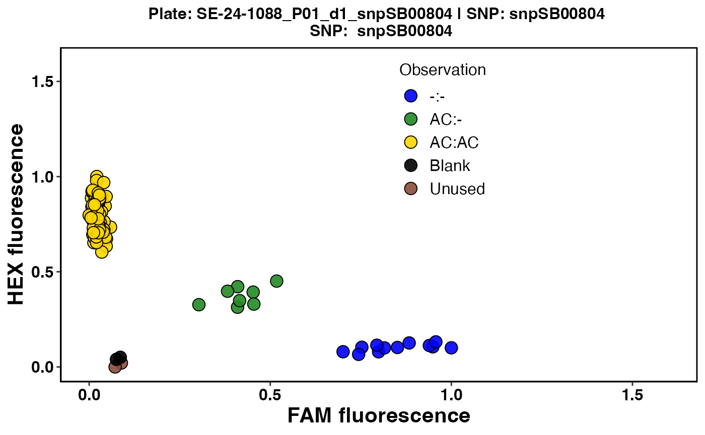

Fig. 3. Cluster plot for Plate 5 using FAM and HEX colors for grouping observed genotypes.

# KASP QC plot for Plate 05
library(panGenomeBreedr)
 kasp_qc_ggplot2(x = dat1[5],
                  pdf = FALSE,
                  Group_id = 'Group',
                  Group_unknown = '?',
                  scale = TRUE,
                  pred_cols = c('Blank' = 'black', 'False' = 'firebrick3',
                              'True' = 'cornflowerblue', 'Unverified' = 'beige'),
                  expand_axis = 0.6,
                  alpha = 0.9,
                  legend.pos.x = 0.6,
                  legend.pos.y = 0.75)
#> $`SE-24-1088_P01_d1_snpSB00804`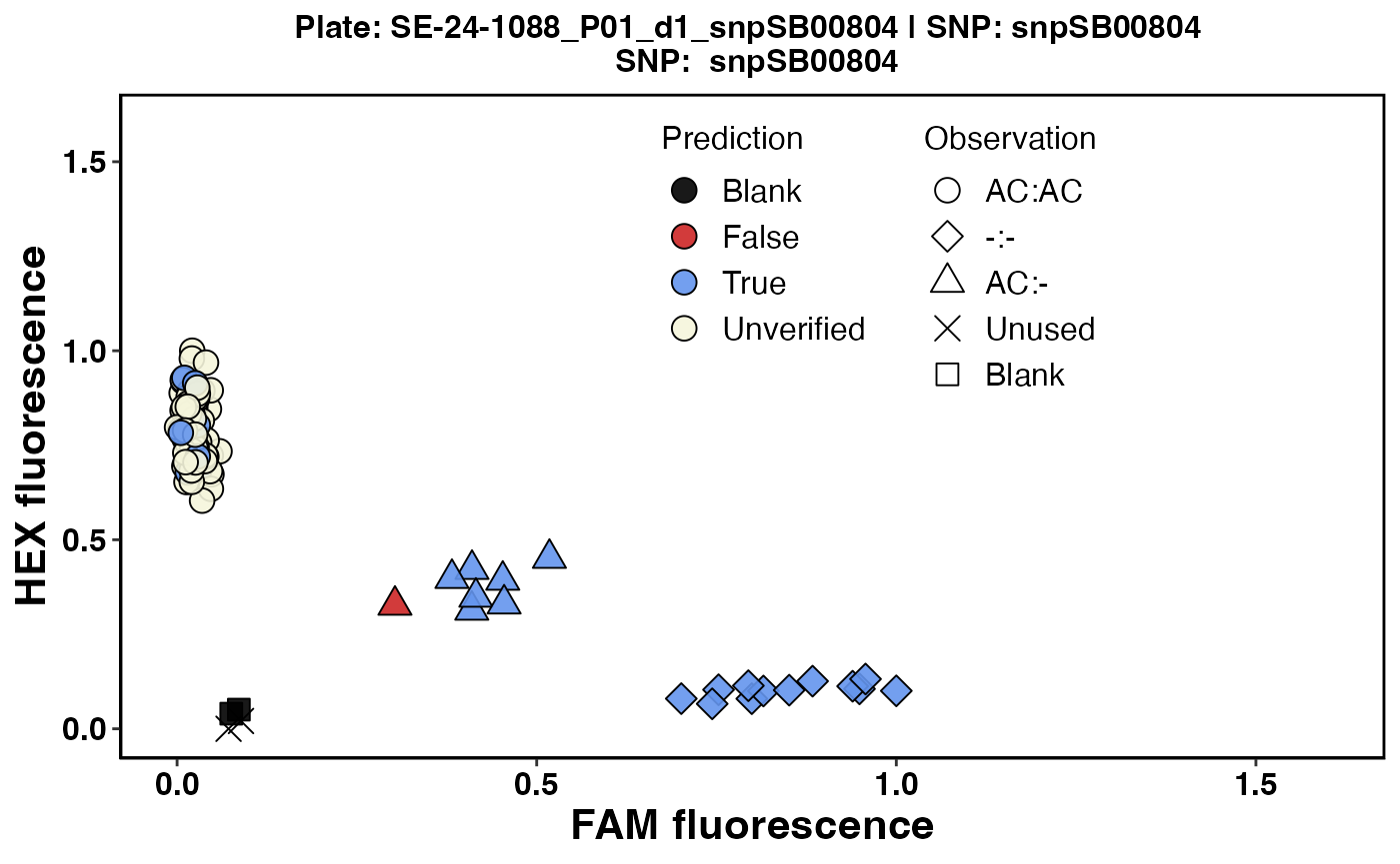

Fig. 4. Cluster plot for Plate 5 with an overlay of predictions for positive controls.

Color-blind-friendly color combinations are used to visualize verified genotype predictions (Figure 3).

In Figure 4, the three genotype classes are grouped based on plot PCH symbols using the FAM and HEX scores for observed genotype calls.

To simplify the verified prediction overlay for the expected genotypes for positive controls, all possible outcomes are divided into three categories (TRUE, FALSE, and UNVERIFIED) and color-coded to make it easier to visualize verified predictions.

BLUE (color code for the TRUE category) means genotype prediction matches the observed genotype call for the sample.

RED (color code for the FALSE category) means genotype prediction does not match the observed genotype call for the sample.

BEIGE (color code for the UNVERIFIED category) means three things: an expected genotype call could not be made before KASP genotyping, or an observed genotype call could not be made to verify the prediction.

Users can set the pdf = TRUE argument to save plots as a PDF file in a directory outside R. The kasp_qc_ggplot() and kasp_qc_ggplot2()functions can generate cluster plots for multiple plates simultaneously.

To visualize predictions for positive controls to validate KASP markers, the column name containing expected genotype calls must be provided and passed to the function using the Group_id = 'Group' argument as shown in the code snippets above. If this information is not available, set the argument Group_id = NULL.

Summary of Prediction Verification in Plates

The pred_summary() function produces a summary of predicted genotypes for positive controls in each reaction plate after verification (Table 3), as shown in the code snippet below:

# Get prediction summary for all plates
library(panGenomeBreedr)
my_sum <- pred_summary(x = dat1,
                       snp_id = 'SNPID',
                       Group_id = 'Group',
                       Group_unknown = '?',
                       geno_call = 'Call',
                       rate_out = TRUE)

Table 3: Summary of verified prediction status for samples in plates

plate	snp_id	false	true	unverified
SE-24-1088_P01_d1_snpSB00800	snpSB00800	0.04	0.06	0.90
SE-24-1088_P01_d2_snpSB00800	snpSB00800	0.02	0.06	0.92
SE-24-1088_P01_d1_snpSB00803	snpSB00803	0.00	0.34	0.66
SE-24-1088_P01_d2_snpSB00803	snpSB00803	0.00	0.34	0.66
SE-24-1088_P01_d1_snpSB00804	snpSB00804	0.01	0.33	0.66
SE-24-1088_P01_d2_snpSB00804	snpSB00804	0.01	0.33	0.66
SE-24-1088_P01_d1_snpSB00805	snpSB00805	0.15	0.19	0.66
SE-24-1088_P01_d2_snpSB00805	snpSB00805	0.15	0.19	0.66

The output of the pred_summary() function can be visualized as bar plots using the pred_summary_plot() function as shown in the code snippet below:

# Get prediction summary for snp:snpSB00804
library(panGenomeBreedr)
my_sum <- my_sum$summ
my_sum <- my_sum[my_sum$snp_id == 'snpSB00804',]

 pred_summary_plot(x = my_sum,
                    pdf = FALSE,
                    pred_cols = c('false' = 'firebrick3', 'true' = 'cornflowerblue',
                                  'unverified' = 'beige'),
                    alpha = 1,
                    text_size = 12,
                    width = 6,
                    height = 6,
                    angle = 45)
#> $snpSB00804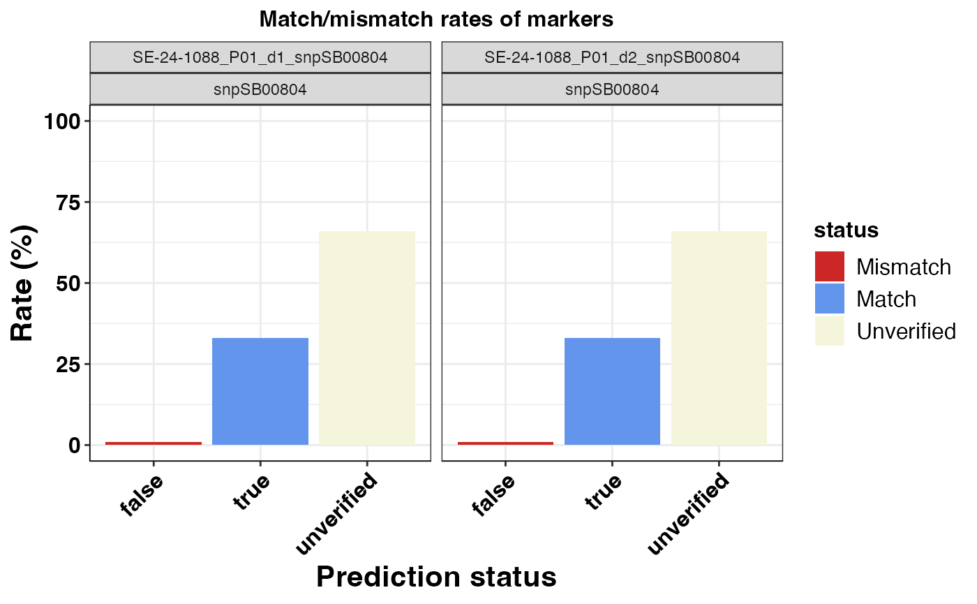

Fig. 5. Match/Mismatch rate of predictions for snp: snpSB00804.

Plot Plate Design

Users can visualize the observed genotype calls in a plate design format using the plot_plate() function as depicted in Figure 5, using the code snippet below:

plot_plate(dat1[5], pdf = FALSE)
#> $`SE-24-1088_P01_d1_snpSB00804`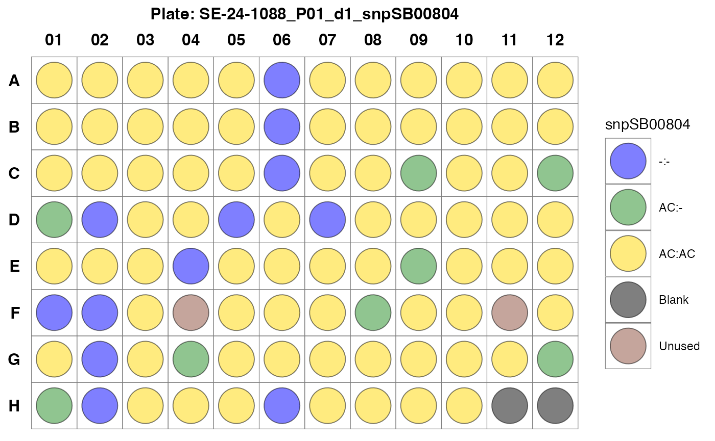

Fig. 6. Observed genotype calls for samples in Plate 5 in a plate design format.

Decision Support for Trait Introgression and MABC

panGB provides additional functionalities to test hypotheses on the success of trait introgression pipelines and crosses.

Users can easily generate heatmaps that compare the genetic background of parents to progenies to ascertain if a target locus was successfully introgressed or check for the hybridity of F1s. These plots also allow users to get a visual insight into the amount of parent germplasm recovered in progenies.

To produce these plots, users must have either polymorphic low or mid-density marker data and a map file for the markers. The map file must contain the marker IDs, their chromosome numbers and positions.

panGBcan handle data from KASP, Agriplex and DArTag service providers.

Working with Agriplex Mid-Density Marker Data

Agriplex data is structurally different from KASP or DArTag data in terms of genotype call coding and formatting. Agriplex uses ' / ' as a separator for genotype calls for heterozygotes, and uses single nucleotides to represent homozygous SNP calls.

Creating Heatmaps with panGB

To exemplify the steps for creating heatmap, we will use a mid-density marker data for three groups of near-isogenic lines (NILs) and their parents (Table 4). The NILs and their parents were genotyped using the Agriplex platform. Each NIL group was genotyped using 2421 markers.

The imported data frame has the markers as columns and genotyped samples as rows. It comes with some meta data about the samples. Marker names are informative: chromosome number and position coordinates are embedded in the marker names (Eg. S1_778962: chr = 1, pos = 779862).

# Set path to the directory where your data is located
path1 <-  system.file("extdata", "agriplex_dat.csv",
                       package = "panGenomeBreedr",
                      mustWork = TRUE)

# Import raw Agriplex data file
geno <- read.csv(file = path1, header = TRUE, colClasses = c("character")) # genotype calls

library(knitr)
knitr::kable(geno[1:6, 1:10], caption = 'Table 4: Agriplex data format', format = 'html', booktabs = TRUE)

Table 4: Agriplex data format

Plate.name	Well	Sample_ID	Batch	Genotype	Status	S1_778962	S1_1019896	S1_1613105	S1_1954298
RHODES_PLATE1	D04	NIL_1	1	RTx430a	Recurrent parent	A	G	G	A
RHODES_PLATE1	F04	NIL_2	1	RTx430b	Recurrent parent	A	G	G	A
RHODES_PLATE1	G04	NIL_3	1	IRAT204a	Donor parent	G	C	G	A
RHODES_PLATE1	A05	NIL_4	1	IRAT204b	Donor Parent	G	C	G	A
RHODES_PLATE1	D07	NIL_5	1	RMES1+|+_1	NIL+	A	G	G	A
RHODES_PLATE1	F08	NIL_6	1	RMES1+|+_2	NIL+	A	G	G	A

To create a heatmap that compares the genetic background of parents and NILs across all markers, we need to first process the raw Agriplex data into a numeric format. The panGB package has customizable data wrangling functions for KASP, Agriplex, and DArTag data.

The rm_mono() function can be used to filter out all monomorphic loci from the data.

Since our imported Agriplex data has informative SNP IDs, we can use the parse_marker_ns() function to generate a map file (Table 5) for the markers.
The generated map file is then passed to the proc_kasp() function to order the SNP markers according to their chromosome numbers and positions.

The kasp_numeric() function converts the output of the proc_kasp() function into a numeric format (Table 6). The re-coding to numeric format is done as follows:

• Homozygous for Parent 1 allele = 1.
• Homozygous for Parent 2 allele = 0.
• Heterozygous = 0.5.
• Monomorphic loci = -1.
• Loci with a suspected genotype error = -2.
• Loci with at least one missing parental or any other genotype = -5.

# Parse snp ids to generate a map file
library(panGenomeBreedr)

# Data for stg5 NILs
stg5 <- geno[geno$Batch == 3, -c(1:6)] 
rownames(stg5) <- geno$Genotype[17:25]

# Remove monomorphic loci from data
stg5 <- rm_mono(stg5)

# Parse snp ids to generate a map file
snps <- colnames(stg5) # Get snp ids
map_file <- parse_marker_ns(x = snps, sep = '_', prefix = 'S')

# order markers in map file
map_file <- order_markers(x = map_file)

Table 5: Map file for the imported Agriplex data.

	snpid	chr	pos
1.317	S1_402592	1	402592
1.1	S1_778962	1	778962
1.633	S1_825853	1	825853
1.318	S1_1218846	1	1218846
1.2	S1_1613105	1	1613105
1.319	S1_1727150	1	1727150
1.3	S1_1954298	1	1954298
1.4	S1_1985365	1	1985365

# Process genotype data to re-order SNPs based on chromosome and positions
stg5 <- proc_kasp(x = stg5,
                  kasp_map = map_file,
                  map_snp_id = "snpid",
                  sample_id = "Genotype",
                  marker_start = 1,
                  chr = 'chr',
                  chr_pos = 'pos')

# Convert to numeric format for plotting
num_geno <- kasp_numeric(x = stg5,
                         rp_row = 1,
                         dp_row = 3,
                         sep = ' / ',
                         data_type = 'agriplex')

Table 6: Agriplex data converted to a numeric format.

	S1_402592	S1_778962	S1_825853	S1_1218846	S1_1613105	S1_1727150	S1_1954298	S1_1985365
BTx623a	1	1	1	1	1	1	1	1
BTx623b	1	1	1	1	1	1	1	1
BTx642a	0	0	0	0	0	0	0	0
BTx642b	0	0	0	0	0	0	0	0
Stg5+|+_1	1	0	0	0	0	0	0	0
Stg5+|+_2	0	0	0	0	0	1	1	1
Stg5-|-_1	1	1	1	1	1	1	1	1
Stg5-|-_2	1	1	1	1	1	1	1	1
Stg5-|-_3	1	1	1	1	1	1	1	1

All is now set to generate the heatmap (Figure 6) using the cross_qc_ggplot() function, as shown in the code snippet below:

# Get prediction summary for snp:snpSB00804
library(panGenomeBreedr)
# Create a heatmap that compares the parents to progenies
cross_qc_heatmap(x = num_geno,
                map_file = map_file,
                snp_ids = 'snpid',
                chr = 'chr',
                chr_pos = 'pos',
                parents = c("BTx623a", "BTx642a"),
                pdf = FALSE,
                filename = 'background_heatmap',
                legend_title = 'stg5_NILs',
                alpha = 0.9,
                text_size = 15)
#> $Batch1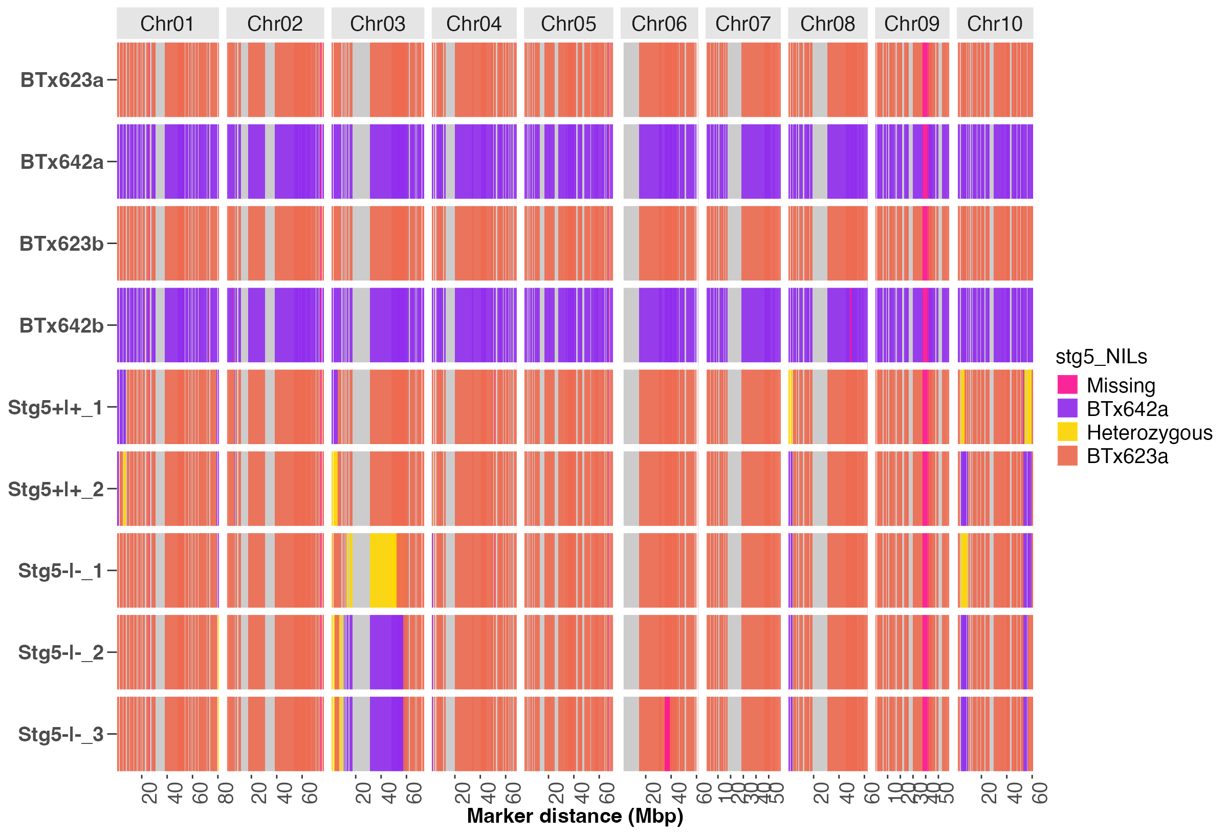

Fig. 6. A heatmap that compares the genetic background of parents and stg5 NIL progenies across all markers.

The cross_qc_ggplot() function is a wrapper for functions in the ggplot2 package.

Users must specify the IDs for the two parents using the parents argument. In the code snippet above, the recurrent parent is BTx623 and the donor parent for the stg5 locus is BTx642.

The group_sz argument must be specified to plot the heatmap in batches of progenies to avoid cluttering the plot with many observations.

Users can set the pdf = TRUE argument to save plots as a PDF file in a directory outside R.

Trait Introgression Hypothesis Testing

To test the hypothesis that the stg5 NIL development was effective, we can use the cross_qc_annotate() function to generate a heatmap (Figure 7) with an annotation of the position of the stg5 locus on Chr 1, as shown below:

###########################################################################
# Subset data for the first 30 markers on Chr 1
stg5_ch1 <- num_geno[, map_file$chr == 1][,1:20] 

# Get the map file for subset data
stg5_ch1_map <- parse_marker_ns(colnames(stg5_ch1))

# Annotate a heatmap to show the stg5 locus on Chr 1
# The locus is between positions 1e6 - 1.4 Mbp on Chr 1
cross_qc_heatmap(x = stg5_ch1,
                  map_file = stg5_ch1_map,
                  snp_ids = 'snpid',
                  chr = 'chr',
                  chr_pos = 'pos',
                  parents = c("BTx623a", "BTx642a"),
                  trait_pos = list(stg5 = c(chr = 1, start = 1e6, end = 1.4e6)),
                  text_scale_fct = 0.18,
                  pdf = FALSE,
                  legend_title = 'Stg5_NILs',
                  alpha = 0.9,
                  text_size = 15)
#> $Batch1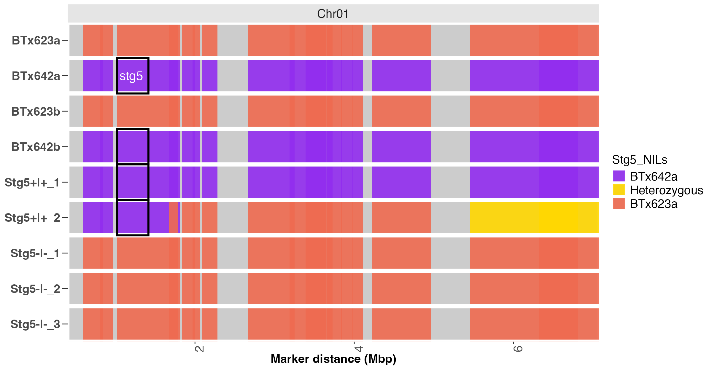

Fig. 7. Heatmap annotation of the stg5 locus on Chr 1.

In the code snippet above, the numeric matrix of genotype calls and its associated map file are required.

The recurrent and donor parents must be specified using the parents argument.

The snp_ids, chr, and chr_pos arguments can be used to specify the column names for marker IDs, chromosome number and positions in the attached map file.
The trait_pos argument was used to specify the position of the target locus (stg5) on chromosome one. Users can specify the positions of multiple target loci as components of a list object for annotation.

In Figure 7, the color intensity correlates positively with the marker density or coverage. Thus, areas with no color (white vertical gaps) depicts gaps in the marker coverage in the data.

Decision Support for MABC

Users can use the calc_rpp_bc() function in panGB to calculate the proportion of recurrent parent background (RPP) fully recovered in backcross progenies.

It also returns the rpp value for each chromosome.

In the computation, partially regions are ignored, hence, heterozygous scores are not used.

The output for he calc_rpp_bc() function can be passed to the rpp_barplot() function to visualize the computed RPP values for progenies as a bar plot. Users can specify an RPP threshold to easily identify lines that have RPP values above or equal to the defined RPP threshold on the bar plot.

We can compute and visualize the observed RPP values for the stg5 NILs across all polymorphic loci as shown in the code snippet below:

# Calculate weighted RPP
rpp <- calc_rpp_bc(x = num_geno,
                   map_file = map_file,
                   map_chr = 'chr',
                   map_pos = 'pos',
                   map_snp_ids = 'snpid',
                   rp = 1,
                   rp_num_code = 1,
                   na_code = -5,
                   weighted = TRUE)

# Generate bar plot for RPP values
rpp_barplot(rpp_df = rpp,
            rpp_threshold = 0.93,
            text_size = 18,
            text_scale_fct = 0.1,
            alpha = 0.9,
            bar_width = 0.5,
            aspect_ratio = 0.5,
            pdf = FALSE)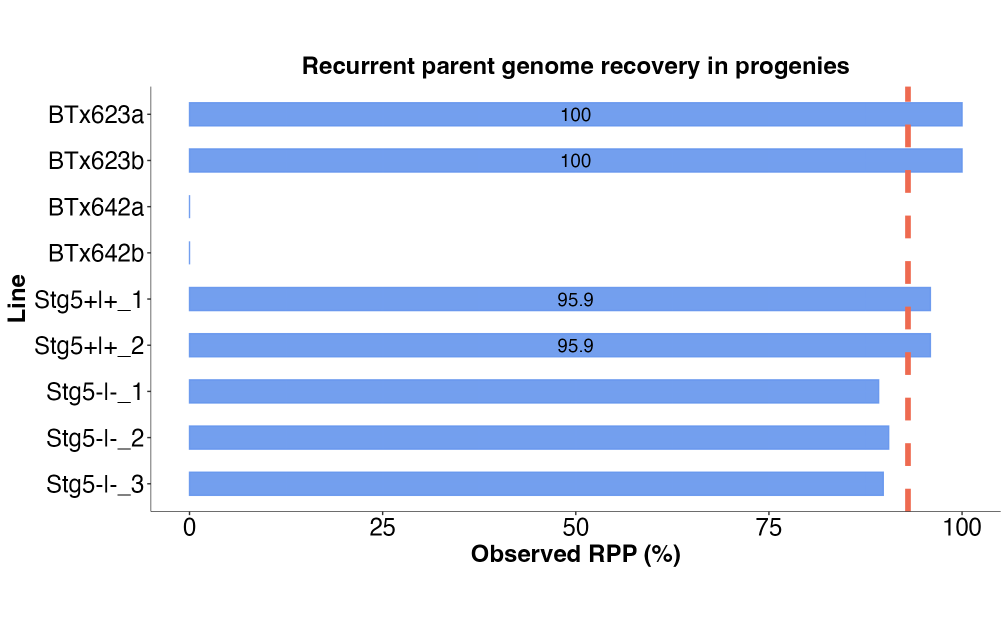

Fig. 8. Computed RPP values for the stg5 NILs.

RPP computation across and for each chromosome.

	sample_id	chr_1	chr_2	chr_3	chr_4	chr_5	chr_6	chr_7	chr_8	chr_9	chr_10	total_rpp
BTx623a	BTx623a	1.000	1.000	1.000	1.000	1	1.000	1	1.000	1	1.000	1.000
BTx623b	BTx623b	1.000	1.000	1.000	1.000	1	1.000	1	1.000	1	1.000	1.000
BTx642a	BTx642a	0.000	0.000	0.000	0.000	0	0.000	0	0.000	0	0.000	0.000
BTx642b	BTx642b	0.000	0.000	0.000	0.000	0	0.000	0	0.000	0	0.000	0.000
Stg5+|+_1	Stg5+|+_1	0.880	0.997	0.931	0.995	1	1.000	1	0.949	1	0.840	0.959
Stg5+|+_2	Stg5+|+_2	0.924	0.997	0.939	0.987	1	1.000	1	0.949	1	0.796	0.959
Stg5-|-_1	Stg5-|-_1	0.982	1.000	0.455	0.984	1	0.759	1	0.949	1	0.796	0.892
Stg5-|-_2	Stg5-|-_2	0.991	1.000	0.286	0.987	1	0.995	1	0.949	1	0.845	0.905
Stg5-|-_3	Stg5-|-_3	0.991	1.000	0.278	0.987	1	0.931	1	0.949	1	0.845	0.898

The calc_rpp_bc() function in panGB provides two algorithms for computing the observed RPP values: weighted and unweighted RPP values. We recommend the use of the weighted algorithm to account for differences in the marker coverage across the genome.

The algorithm for the weighted RPP values is explained below.

Weighted RPP Computation in panGB

Let $w_i$ represent the weight for marker $i$, based on the relative distances to its adjacent markers.

For a set of markers with positions $p_1, p_2, \ldots, p_n$, where $d_i = p_{i+1} - p_i$ represents the distance between adjacent markers, the weights can be calculated as follows:

1. For the first marker $i = 1$:

   $$w_1 = \frac{d_1}{2 \sum_{i=1}^{n-1} d_i}$$

2. For a middle marker $1 < i < n$:

   $$w_i = \frac{d_{i-1} + d_i}{2 \sum_{i=1}^{n-1} d_i}$$

3. For the last marker $i = n$:

   $$w_n = \frac{d_{n-1}}{2 \sum_{i=1}^{n-1} d_i}$$

where:

• $d_i$ is the distance between marker $i$ and marker $i+1$,
• $sum_{i=1}^{n-1} d_i$ is the total distance across all segments, used for normalization.

Let $RPP$ represent the Recurrent Parent Proportion based on relative distance weighting. If $w_i$ is the weight for each marker $i$, and $m_i$ represents whether marker $i$ matches the recurrent parent $m_i = 1$ if it matches, $m_i = 0$ otherwise), then the weighted RPP is calculated as:

$$RPP_{weighted} = \sum_{i=1}^n w_i\cdot m_i$$

The unweighted RPP is calculated without the use of the weights as follows:

$$RPP_{unweighted} = \frac{\sum_{i=1}^n m_i} n$$

where:

• $w_i$ is the weight of marker $i$, calculated based on the relative distance it covers,
• $m_i$ is the match indicator for marker $i$ (1 if matching the recurrent parent, 0 otherwise),
• $n$ is the total number of markers.

This formula provides the sum of the weighted contributions from each marker, representing the proportion of the recurrent parent genome in the individual.

Decision Support for Foreground Selection

The foreground_select() and find_lines() functions are designed to help breeders identify lines that carry favorable alleles at target loci using trait-predictive markers. This process supports foreground selection in marker-assisted selection pipelines.

Generate a Binary Matrix: foreground_select() function

The foreground_select() function score Lines for presence of favorable alleles by converting raw marker genotype data into a binary matrix (1 = favorable allele present, 0 = absent) based on a set of trait-predictive markers. The foreground_select() function is shown in the code snippet below:

library(panGenomeBreedr)

# Marker genotype data
geno <- data.frame(SNP1 = c("A:A", "A:G", "G:G", "A:A"),
                   SNP2 = c("C:C", "C:T", "T:T", "C:T"),
                   SNP3 = c("G:G", "G:G", "A:G", "A:A"),
                   row.names = c("Line1", "Line2", "Line3", "Line4"))

# Trait-predictive marker metadata
marker_info <- data.frame(qtl_markers = paste0("SNP", 1:3),
                           locus_name = paste0('loc', 1:3),
                          fav_alleles = c("A", "C", "G"),
                         
                          alt_alleles = c("G", "T", "A"))

# Convert raw genotypes to binary (foreground profile)
foreground_matrix <- foreground_select(geno_data = geno,
                                       fore_marker_info = marker_info,
                                       fore_marker_col = "qtl_markers",
                                       fav_allele_col = "fav_alleles",
                                       alt_allele_col = "alt_alleles",
                                       select_type = "homo")

Binary matrix of presence or absence of favorable alleles.

	SNP1	SNP2	SNP3
Line1	1	1	1
Line2	0	0	1
Line3	0	0	0
Line4	1	0	0

The foreground_select() function has the following input parameters:

Argument	Type	Description
geno_data	data.frame	Marker genotype data (lines x markers), e.g., "A:A", "A:G"
fore_marker_info	data.frame	Metadata describing trait-predictive markers, including marker names, favorable alleles, and alternate alleles
fore_marker_col	character	Column name in fore_marker_info for marker names
fav_allele_col	character	Column name for favorable allele
alt_allele_col	character	Column name for alternate allele
select_type	character	Genotype class to select: "homo", "hetero", or "both"
sep	character	Separator used in genotype calls (e.g., ":")

Visualize the Binary Data with UpSet Plot

Generate an UpSet plot using the UpSetR package to explore the co-occurrence of favorable alleles across lines. The UpSet plot allows users to quickly determine:

• Whether any line carries favorable alleles at all target loci.

• How favorable alleles are distributed across lines.

• Which loci are rarely combined.

How to Interpret the UpSet Plot:

• Top bar plot: shows the number of lines for each unique combination (intersection) of target loci with favorable alleles.

• Bottom matrix of dots and lines: indicates which loci are involved in each combination.

• Left bar plot: shows how many lines have the favorable allele for each individual target locus.

# Make an Upset plot and overlay with trait loci names
metadata <- data.frame(sets = marker_info$qtl_markers,
                      locus = marker_info$locus_name)

nl <- ncol(foreground_matrix) # Number of markers

UpSetR::upset(foreground_matrix,
              nsets = nl,
              mainbar.y.label = "Locus Intersection Size",
              sets.x.label = "Locus Size",
              text.scale = 1.2,
              set.metadata = list(data = metadata,
                          plots = list(list(type = 'text', 
                                            assign = 8,
                                            column = 'locus',
                                            colors = rep('firebrick2', nl)))))

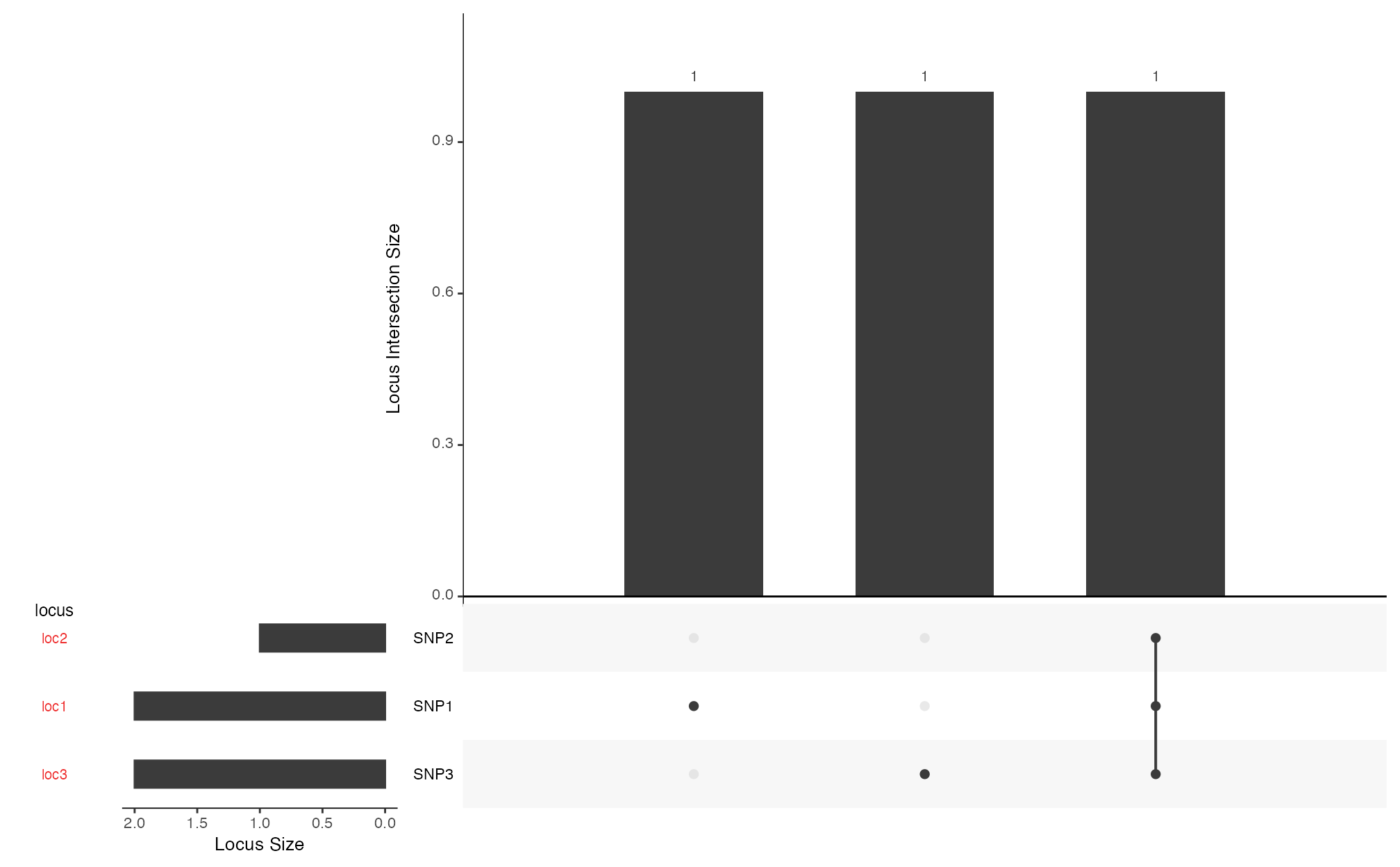
Fig. 9. Visualizing the co-occurrence of favorable alleles across lines.

Query Lines by Intersection Category: find_lines() function

The find_lines() function identifies lines based on target loci profile by filtering the binary output of foreground_select() to return line names that match a desired allele presence/absence profile across loci. Using the binary matrix, users can extract line IDs corresponding to any intersection (i.e., specific combinations of favorable alleles revealed by the UpSet plot).

library(panGenomeBreedr)

# Find lines with favorable alleles at all target loci
selected_lines <- find_lines(mat = foreground_matrix,
                             present = c('SNP1', 'SNP2', 'SNP3'))

print(selected_lines)
#> [1] "Line1"

The find_lines() function has the following input parameters:

Argument	Type	Description
mat	data.frame	Binary matrix.
present	character	Markers that must be 1.
absent	character	Markers that must be 0.

Troubleshooting

If the package does not run as expected, check the following:

• Was the package properly installed?

• Do you have the required dependencies installed?

• Were any warnings or error messages returned during package installation?

• Are all packages up to date before installing panGB?

Authors and contributors

• Alexander Wireko Kena

• Israel Tawiah Tetteh

• Cruet Burgos

• Linly Banda

• Jacques Faye

• Fanna Maina

• Terry Felderhoff

• Geoffrey Preston Morris

License

GNU GPLv3

Support and Feedback

For support and submission of feedback, email the maintainer Alexander Kena, PhD at alex.kena24@gmail.com